Neural Network Sandbox
August 2025
Abstract
Developed a simple way to create different Artificial Neural Networks (ANN/NN) architectures seeking to reduce programmatic overhead, while improving efficiency over popular python-based frameworks such as TensorFlow or PyTorch. This was achieved by leveraging the low-level performance and memory-safety features that Rust provides.
Project Requirement
-
The system must be scalable.
-
Implement a way to define the desired architecture for a Feed-Forward Deep Neural Network.
-
Allow for the user to define a desired number of input neurons.
-
Allow for the user to define a desired number of hidden layers.
-
Allow for the user to define a desired number of neurons per hidden layer.
-
Allow for the user to define a desired number of output neurons.
-
Allow for the user to define a desired activation function for a given hidden layer.
-
Allow for the user to define a desired activation function for the output layer.
-
Allow for the user to easily train the neural network.
-
Allow for the system to determine the optimal back-propagation calculations during training.
-
Allow for the user to easily test the neural network.
-
Allow for the neural network to be saved in a standardized format.
-
Identify training time elapsed for benchmarking.
-
Identify training resource utilization for benchmarking.
What is a Machine Learning?
Machine Learning is a field of study within artificial intelligence concerned with the development and study of statistical algorithms that can learn from data and generalize to unseen data, to perform tasks without explicit instruction.
There are three main approaches to the development of these statistical models:
Supervised Learning (SL)
Unsupervised Learning (UL)
-
Classification
-
Regression
-
Clustering
-
Association
-
Dimensionality Reduction
-
Feature Learning
-
Density Estimation
-
Generative Models
Reinforcement Learning (RL)
-
Stochasticity
-
Credit Assignment Problem
-
Non-differentiability
These approaches are mainly driven by the nature of the available data, the type of task or problem being solved, and the specific goals of the learning process.
There are many other types of algorithms that can be used to solve SL, UL, and RL problems. However, Neural Networks are the preferred approach due to their advantages in problem complexity scalability, generalization, and computational parallelization.
What is a Neural Network?
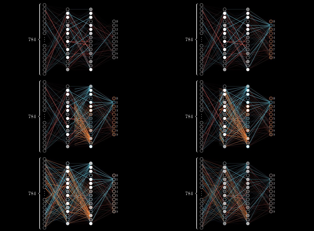
A neural network is a type of machine learning model inspired by the structure of the human brain. It’s designed to recognize patterns, make predictions, and learn from data.
At its core, a neural network consists of layers of interconnected nodes (called neurons), each performing simple mathematical operations. These neurons work together to transform input data (like an image or a sentence) into meaningful output (such as identifying a cat or translating a phrase).
How Does It Work?
-
Input Layer: This is where data enters the network. Each input is represented as a number.
-
Hidden Layers: These layers process the data through weighted connections and activation functions. The network adjusts these weights during training to improve accuracy.
-
Output Layer: This layer produces the final result—whether it’s a classification, a prediction, or a decision.
What is a Neuron?
The neurons used in modern NNs have their origin in a concept invented in 1943, The Perceptron. This is a classification algorithm makes its predictions based on a linear predictor function combining a weights vector, w, with the feature (input) vector, x, and some offset bias, w_0. These weights and biases acts as dials and knobs to adjust the algorithm to get the desired output given some input. The modern perceptron in NN applications is then fed through an activation function to provide some non-linearity to the approximation, although a linear activation function can be chosen to retain that functionality.

Why Non-linearity?
Non-linearity is necessary for any tasks that require differentiation of items that are not linearly separable. For a simple example, if we wanted to estimate the decision boundary of the logical OR operator, a single line could divide two regions the output can be. This means that the logical OR operator is linearly separable. Alternatively, if we wanted to estimate the decision boundary of the logical XOR operator, two lines would be needed to divide the two regions the output can be in. This means that the logical XOR operator is NOT linearly separable. It is because of this simple example that the XOR became the proof-of-concept for neural networks to be ablet to achieve higher dimensional (more complex) boundary lines.

The choice of activation function is primarily driven by the computational efficiency, the desired gradient behavior during training, the need for non-linearity, and the required range/interpretation for the specific layer or task. See some of the popularly used activation functions below.

How does the Neural Network do anything?
Answer: Forward Propagation
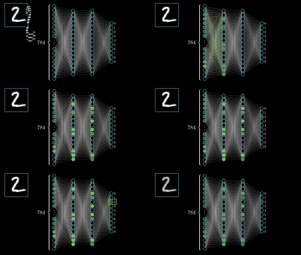
Now that we understand the general structure of a Neural Network and what a neuron does, how does this come together to achieve anything valuable? The answer: Forward Propagation. Forward Propagation is the simple task of taking the inputs (from the input layer) and computing the output for each of the neurons (as described earlier) per layer starting at the first hidden layer, and propagating forward to the output layer.
This, however, is only useful, if the weights and biases have been properly determined to achieve the desired results. Otherwise, we may have the best curated data input, but our network will output garbage.
So, how does the Neural Network learn anything?
Answer: Backward Propagation
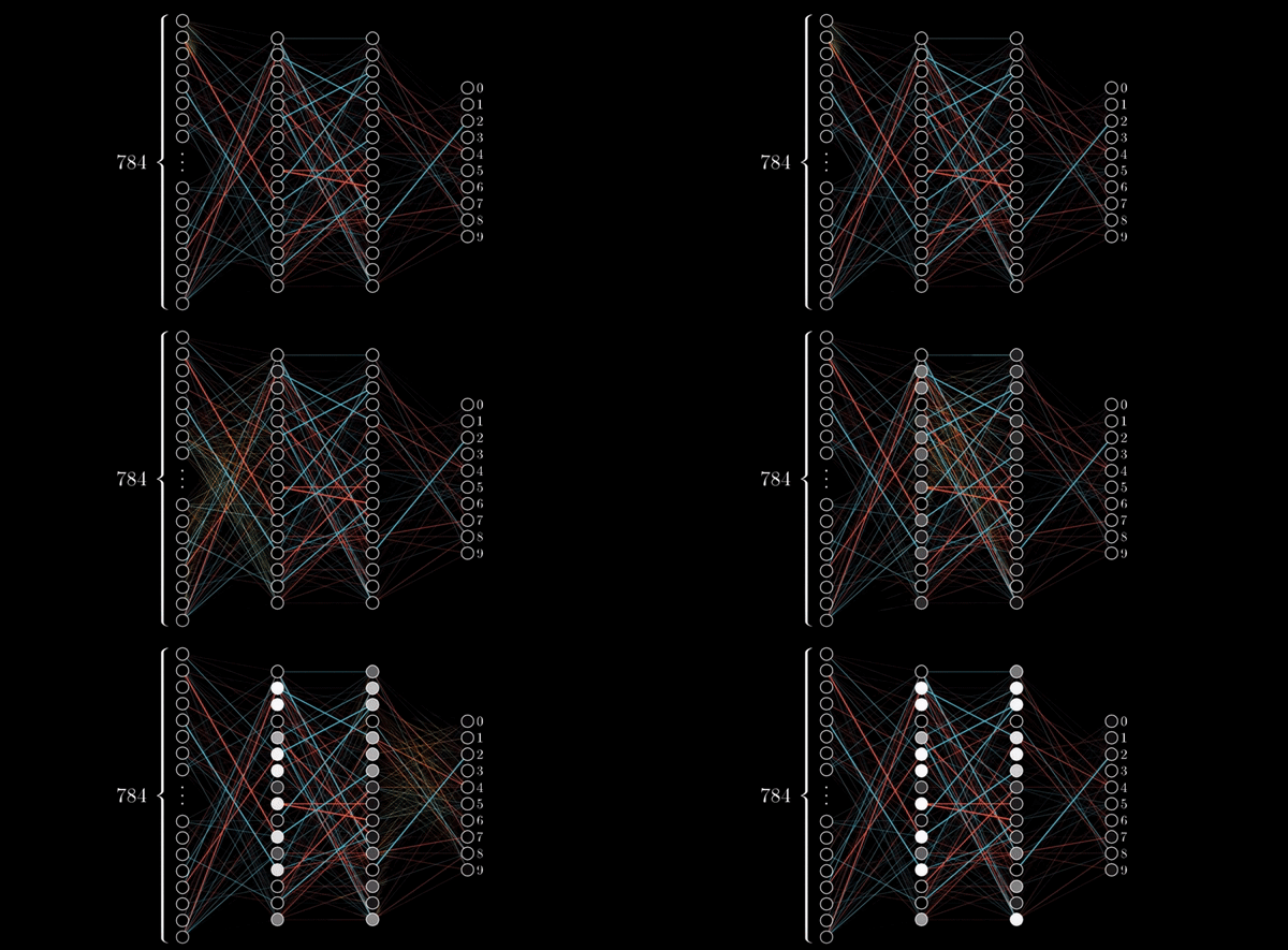
Now, instead of going through every weight vector and bias for each neuron, we can implement a tried and tested method for adjusting these knobs and dials. This process is called back propagation.
The first thing to understand is how does to network know when it's wrong? For this, a Cost Function or Loss Function is implemented. This function choice is dependent on the data available, and application of the network. In short if provides a simple numerical value for how "wrong" an output is given some input.
For example, say we have a NN whose task is to categorize images between cats and dogs. If we feed a picture of a dog, and the NN outputs "cat" it is clearly wrong, so our Loss function may give a result of 1 (or some other arbitrary value dependent on our choice of function). Alternatively, if the output were correct by saying "dog" our Loss function may give a result of 0. This is because there is no error.
With that, our goal is to minimize the loss (error) between our expected value and our actual value. However, the question stands; how do we adjust our weights and biases to reduce the loss? This loss function can be visualized as a hyper-space known as a loss landscape. The loss at a given moment represents some location in this landscape.
This hyper-space is hard to visualize at the dimensions that many NNs operate at, so a 3D visual is used. Now we must figure out how (and by how much) to adjust the weights and biases to navigate this landscape to find a minimum loss.
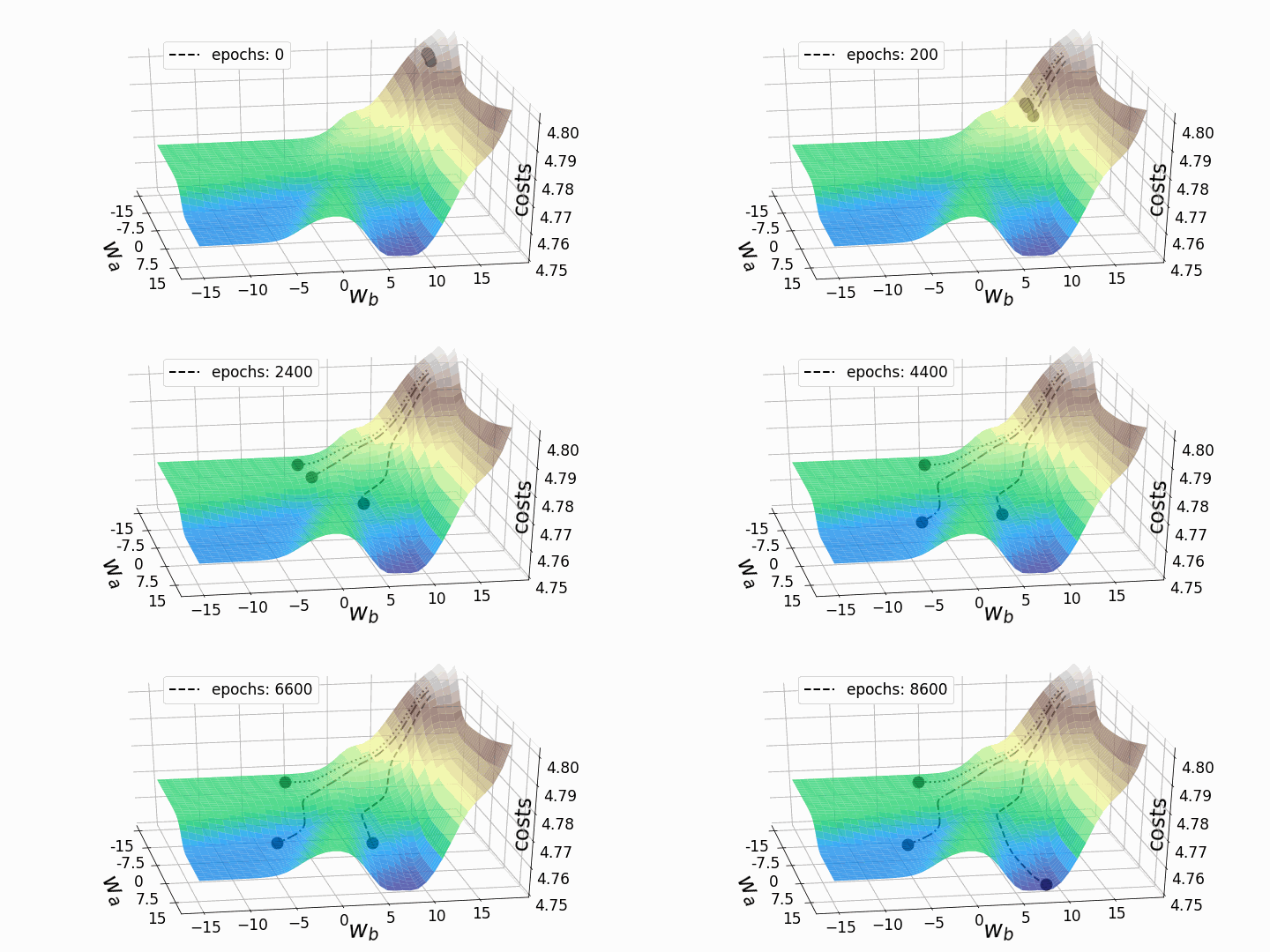
This can be achieved by taking the partial derivative of the output with respect to each of the weights and biases. This tells us in which direction and by how much each weight and bias should be modified to minimize the loss.
The intuition lies in asking the question "If I move my weight by x amount, how much will the output of my network be affected?" This is achieved by performing the chain rule, and localizing the derivative calculations at each neuron.
The equations shown on the right are the partial derivative of the loss function with respect to a given weight. This is determined via known partial derivatives and performing the chain rule to determine the output.

See the animation below. This shows the intuitive approach taken. Where C0 is the cost function that must be minimized, a(L) is the output of the neuron after the activation function, z(L) is the output of the neuron before the activation function a(L-1) is the input from some neuron from a previous layer, w(L) is the weight of the given connection, and b(L) is the bias corresponding to the neuron at hand.
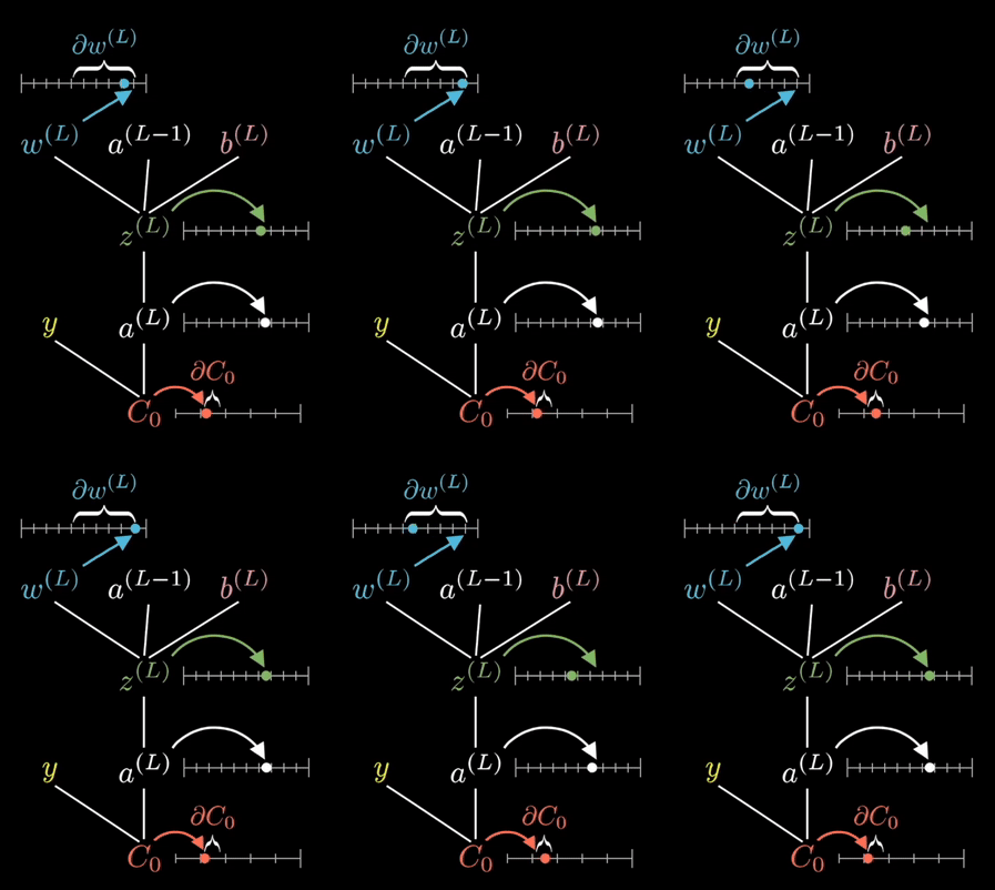
Now this process is repeated for all neurons in the network, and the weights and biases are updated proportionally to how much these contribute to reducing the loss function.
My Approach
Interactive Demo
What's Next?
One of the things I would like to expand on this project is modularizing the codebase. The current version is a monolith, and although functional for my application and testing, I want this to scale.
Additionally, I would like to test its performance on the simple MNIST dataset and explore how this framework can be scaled for more generic architectures that aren't feed-forward networks.
